Computational tutorial

Beginners should start with installation and the simplified cell-gating example. Advanced users can proceed to the advanced tutorial and download five plates of data to process with Dye Drop.

Installation

Open a terminal of your choice.

Clone the github repository

  $ git clone https://github.com/datarail/DrugResponse.git

Install the dependencies:

  $ cd DrugResponse/python
  $ pip install -e .

Cell-gating example

cd into the example folder: cd DrugResponse/python/cell_cycle_gating/examples/
- The example directory (located in DrugResponse/python/cell_cycle_gating/examples/) contains a Raw data folder EX_01[78956].
- This folder contains 10 .txt files, each corresponding to single cell data from a given well (wells C3 to C12).
Type python to open a python terminal or open the Jupyter notebook DDR_example.ipynb and execute the steps in the notebook.

* Based on the python version, you may need to use python3 or other similar commands to launch the terminal. Check with the documentatation of your python distribution to be sure.

The code is reproduced below with a summary of each step.
The example script will: 1) read the contents of the folder, 2) perform automated gating, and 3) output a .csv file and .pdf file that contain well-level summaries of number of live/dead cells and fraction of cells in diferent phases of the cell cycle. In addition, a pdf file containing figures that show the gating per well is available for review.
This example dataset contains 10 wells and should run within a minute. An entire plate with ~300 wells is expected to run in 10-15 minutes.

Running the example

Import required dependencies

  from cell_cycle_gating import run_cell_cycle_gating as rccg ## main cell-gating functions
  import pandas as pd     
  import warnings
  warnings.filterwarnings('ignore')

Import the metadata file that containg mapping between the well name and conditions (i.e cell line, drug, concentration etc).
- Note: a metadata file in not required for succesfully running the script but is highly recommended.
```
  dfm = pd.read_csv('EX_01_metadata.csv')
```
Specify the name of the folder containing the object level data.
- Note: If your data is saved in a single file, provide the name of the file (or entire path).
```
  obj = 'EX_01[78956]'
```
Map user-defined channel names to standarized names required by the script.
- Note: The column names in your input dataset may vary based on your software or personal preferences. However, the script expects a set of standard column names for DNA content, LDR, EDU features.
```
  ndict = {'Nuclei Selected - EdUINT': 'edu',
       'Nuclei Selected - DNAcontent': 'dna',
       'Nuclei Selected - LDRTXT SER Spot 8 px': 'ldrint',
       'Nuclei Selected - pH3INT': 'ph3'}
```
Run automated gating on the example dataset. (Run time ~1 minute)
```
  dfs = rccg.run(obj, ndict, dfm)
```

dfs is data frame that will be returned containing well-level summary of live/dead and fraction of cells in S, G1, G2 M, etc.
Two files summary_EX_01[78956].csv and summary_EX_01[78956].pdf will be saved in a new results/ folder in your local directory.
- EX_01[78956].csv - A comma-separated text file with a table containing rows corresponding to wells in the 96 well plate.
  Each row contains a well-level summary of the number of live/dead cells and fraction of cells in each phase of the cell cycle for one well.

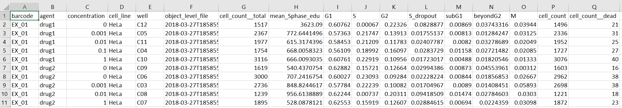Example .csv output table Example output table

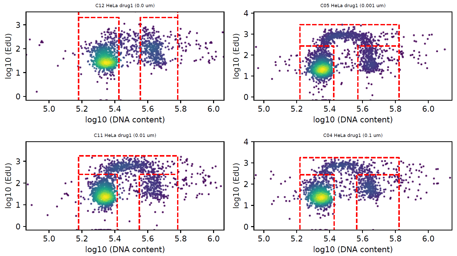Example output figurese Example output figures

Advanced example

We have deposited two additional Jupyter notebooks and five plates of example data on Synapse for download - you will need to make a free Synapse account in order to download this data.

With the first Jupyter notebook, 1-cell_cycle_gating.ipynb, you will run cell cycle analysis on these data. The second notebook, 2-cell cycle summary and gr calcs.ipynb, will produce cell cycle summary plots and will calculate GR metrics on the data.

We hope these examples will clarify how Dye Drop can be applied to real-world multi-well plate datasets.