Dye Drop Computational Protocol
Automated gating of single cell Deep Dye Drop data
Dye drop analyzes single-cell feature data automatically with custom scripts. Cell cycle states, such as cell death, G1, G2, S, and M-phase, are determined based on LDR, DNA content, EdU, and pH3 levels using the heuristics described below.
1.) Classification of dead versus live cells based on LDR signal intensity
- LDR intensity values were log transformed [code]
- A kernel density estimate smoothing function was applied to the log transformed data (
seabon.kdeplot)[code] - Using the additive inverse of the smoothened data, the peak of the signal was identified. (
scipy.signal.find_peaks). The corresponding location of the peak on the x-axis corresponds to the LDR intensity cutoff above which cells were considered LDR positive. [code] - Based on empirical data, any peaks at log10LDR < 1.2 were excluded as erroneous peak detections [code]
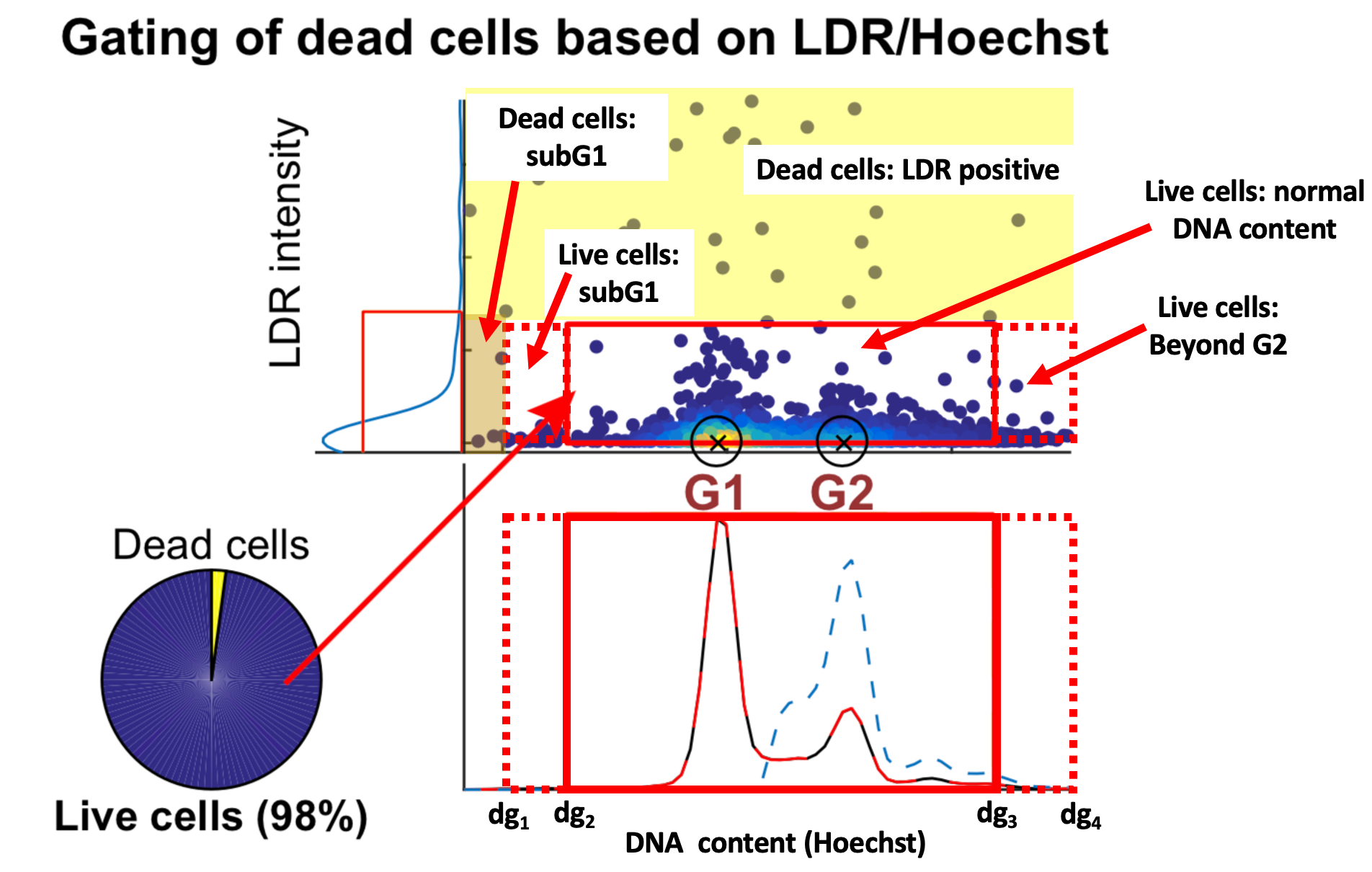
2.) Classification of cells with normal DNA content
- DNA content values were log transformed [code]
- Cells identified as LDR positive in step 1 were excluded (dead cells) and a kernel density smoothing function was applied to log-transformed data.[code]
- A peak finding algorithm was applied to identify all peaks that had a minimal amplitude/height of greater than 10% of maximum
- If only 2 peaks were detected, the minimum of their corresponding x-axis locations (i.e. DNA content) was defined as the approximate G1 peak location. The maximum was defined as the G2 peak location. [code]
- If more than 2 peaks were identified, the peak with the most surrounding DNA density was chosen as the G1 peak location (G1loc).
- To find the location of the G2 peak, the cells with DNA content <= G1 peak location were excluded and the remaining signal was used to identify the local maxima as corresponding to the G1 peak (G2loc)[code]
- Based on empirical assessment, the inner and outer boundaries or gates (dg1 to dg4) were applied [code] as follows:
dg1 = G1loc – 1.5 * (G1loc – G2loc)
dg2 = G1loc – 0.9 * (G1loc – G2loc )
dg3 = G2loc + 1.3 * (G1loc – G2loc )
dg4 = G2loc + 2.2 * (G1loc – G2loc)
- Cells within the inner gates (dg2 < DNA content < dg3) were defined as having normal DNA content. Cells with DNA content between inner and outer left gate are subG1 (dg1 < DNA content < dg2) , cells with DNA content beyond inner right are defined as beyond G2 (DNA content > dg3). Cells with LDR positive status or with DNA content below inner left gate (DNA content < dg1) are defined as dead cells [code]
3.) Classification of cells with high EdU as S-phase cells [code]
- EdU intensity values were log transformed
- A kernel density estimate smoothing function was applied to the log transformed data (
seabon.kdeplot). - Using the additive inverse of the smoothened data, the peak of the signal was identified. (
scipy.signal.find_peaks). The corresponding location of the peak on the x-axis corresponded to the LDR intensity cutoff above which cells were considered EdU high positive.
4.) Using DNA content and EDU signal to identify location of G1, G2 and S phase peak
- EdU intensity values an DNA content were log-transformed
- A 2D histogram EdU and DNA content was computed. [code]
- MATLAB’s
imregionalfunction was used to identify regional maximas on the 2D plate [code] - The regional maximas were used to define a set of candidate peaks for G1, S, and G2 phases. [code]
- Using the individual signal intensity values from EdU and DNA content, the position of G1, S, and G2 peaks were identified using scipy’s peak detection algorithm on the smoothed log values. In the event of multiple peaks identified, the peak which overlapped with the candidate peaks identified in step 4d was selected as the most likely position of the G1, S and G2 foci. [code]
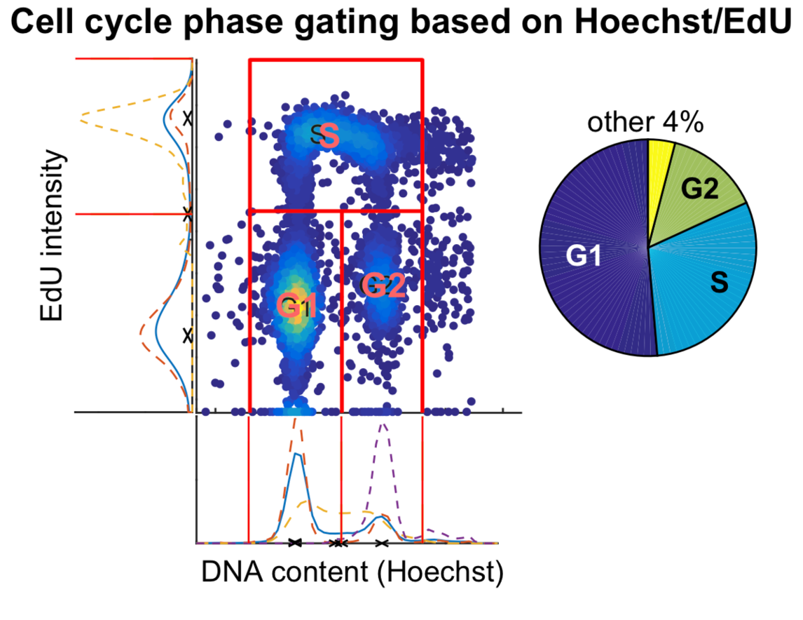
5.) Classification of cells in G1, G2, and S phase
- Cells with EdU content above EdU cutoff were categorized as being in the S-phase
- The remaining cells were carried forward for further classification in G1/G2 phase
- A normal distribution was fit to all cells within the local neighborhood of G1 location identified in Step 4. The boundary between G1 and G2 cells (or S-phase dropout) was defined as X-axis point which lies at the 99% significance interval of the standard distribution. [code]
- Similarly, a normal distribution was fit to all cells within the local neighborhood of G2 location (identified in Step 4). The boundary between G2 and G1 cells (or S-phase dropout) was defined as the X-axis point point which lies at the 1% significance interval of the standard normal distribution.[code]
- Cells whose DNA content fell between the boundaries defined in step 5c & d (if any) were identified as
S-phase dropoutcells. [code]
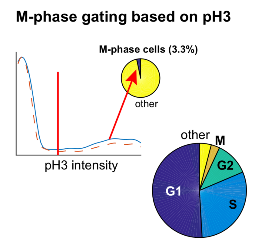
6.) Classification of cells with high pH3 as M-phase cells
- pH3 intensity values were log transformed for all cells evaluated as alive in Step 3h.
- A kernel density estimate smoothing function was applied to the log transformed data. [code]
- Using the additive inverse of the smoothened data, the peak of the signal was identified. (
scipy.signal.find_peaks). The corresponding location of the peak on the x-axis corresponded to the pH3 intensity cutoff above which cells were considered pH3 high positive. - Cells were reclassified as M-phase cells if they passed the criterion in Step 6c. If not, they retained their classification as evaluated in Step 5d-e. [code]