Computational Method
Table of contents
Step 1: Stitching
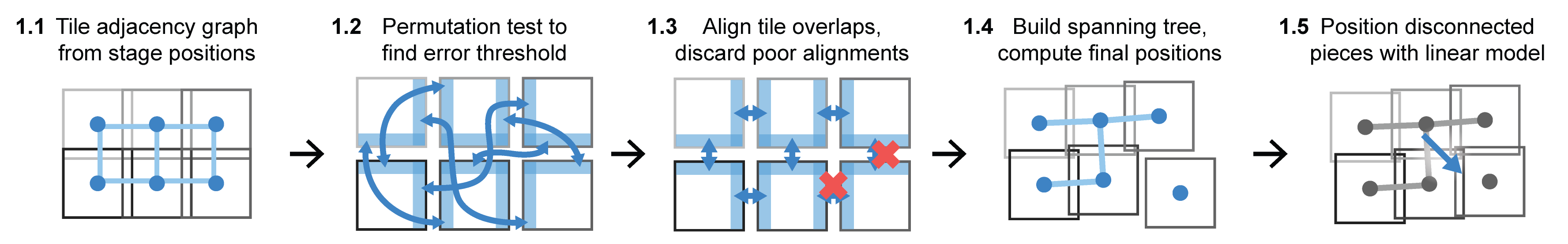
1.1: Tile adjacency graph from stage positions
The stitching procedure starts by creating a node-edge adjacency graph where nodes represent tiles. Edges are added to the graph to connect overlapping tile pairs. Overlapping tile pairs are identified by consulting recorded stage positions and other metadata. Recorded stage positions can be read directly from BioFormats metadata; therefore, it is straightforward to support samples imaged with non-rectangular grids and irregular layouts.
1.2: Permutation test to find error threshold
We use normalized cross correlation (NCC) to score how well the translation returned by phase correlation aligns images, but the threshold dividing an effective alignment from a spurious one varies by data set. We estimate this threshold by the 99th percentile of NCC values computed from a permutation test that considers 1,000 randomly selected pairs of non-adjacent tiles; this corresponds to the unadjusted one-sided empirical p-value threshold of 0.01
1.3: Align tile overlaps, discard poor alignments
We use the negative logarithm of NCC values (referred to as ENCC for NCC error) and a user-provided translation limit parameter to determine whether to accept or discard an alignment of tile pairs. The user-defined value of the translation limit is not particularly critical, as physical translation distances for spurious alignments tend to be extreme. When an alignment is discarded, we delete the corresponding edge from the adjacency graph.
1.4: Build spanning tree, compute final positions
To eliminate graph cycles (loops) from the adjacency graph, a minimum spanning tree is constructed with the ENCC values as the edge weights. We perform the spanning tree procedure independently for each piece in case the edge deletion process in step A3 splits the graph into multiple disconnected pieces. It is then straightforward to walk along the graph from tile to tile, adding up each pairwise alignment along the way to obtain final corrected positions.
1.5: Position disconnected pieces with linear model
In images where step 1.3 splits the adjacency graph into multiple pieces, we adjust the relative positions of disconnected pieces by extrapolating from known-good tile positions using a linear regression model.
Step 2: Registration
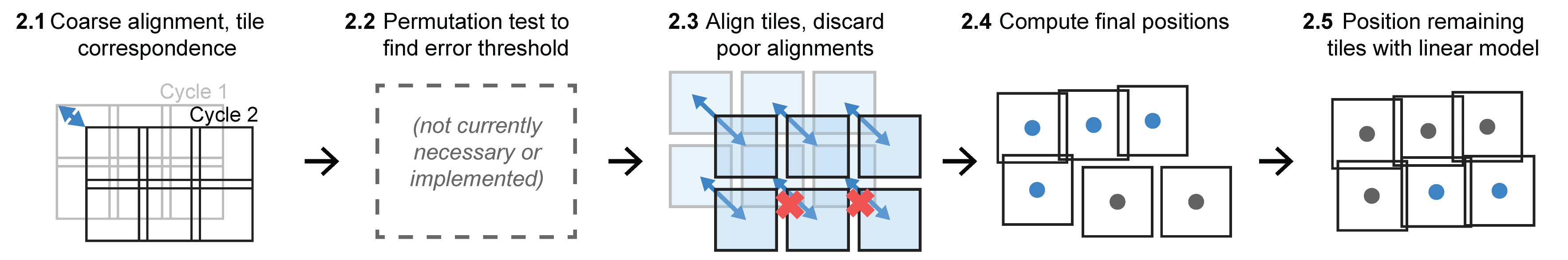
2.1: Coarse alignment, tile correspondence
First we establish a coarse alignment, or correspondence, between each tile in the target cycle (the one to be registered) and the nearest tile in the first cycle by comparing recorded stage positions. Identifying tile correspondences is trivial when recorded stage positions are consistent from run to run and the geometry of the image acquisition grids is identical. However, a significant shift in stage positions between cycles is often introduced by microscopes that lack a physical “homing” procedure to zero stage position encoders at start-up. Shifts also arise if the planned tile grid is significantly displaced or rearranged between runs. To account for this shift when comparing tile positions, we down-sample the data by a factor of 20 and assemble low-resolution “thumbnail” mosaic images for each cycle using the recorded stage positions. We then align the thumbnails using phase correlation with sub-pixel precision to obtain a coarse alignment between the first and target cycles. Working with low-resolution images in this step saves compute time and memory while providing sufficient precision to accurately recover inter-cycle tile correspondences.
2.2: Permutation test to find error threshold
We do not currently use a permutation test and error threshold in the registration phase because the translation limit alone has been sufficient for all images processed to date.
2.3: Align tiles, discard poor alignments
Each corresponding tile pair is cropped to mutually overlapping regions and aligned using phase correlation. The resulting alignments are then filtered using the user- specified translation limit.
2.4: Compute final positions
For alignments that pass the filter, tiles from the target-cycle are positioned by adding the alignment translations to the corrected positions of the corresponding tiles from the first cycle.
2.5: Position remaining tiles with linear model
The remaining tiles (generally those with sparse or no tissue, or where the tissue was damaged significantly during inter-cycle sample handling) are positioned using the linear regression model constructed in the stitching phase.
The result of the stitching and registration phases is a corrected global position for every image tile.
Step 3: Mosaic Image Generation
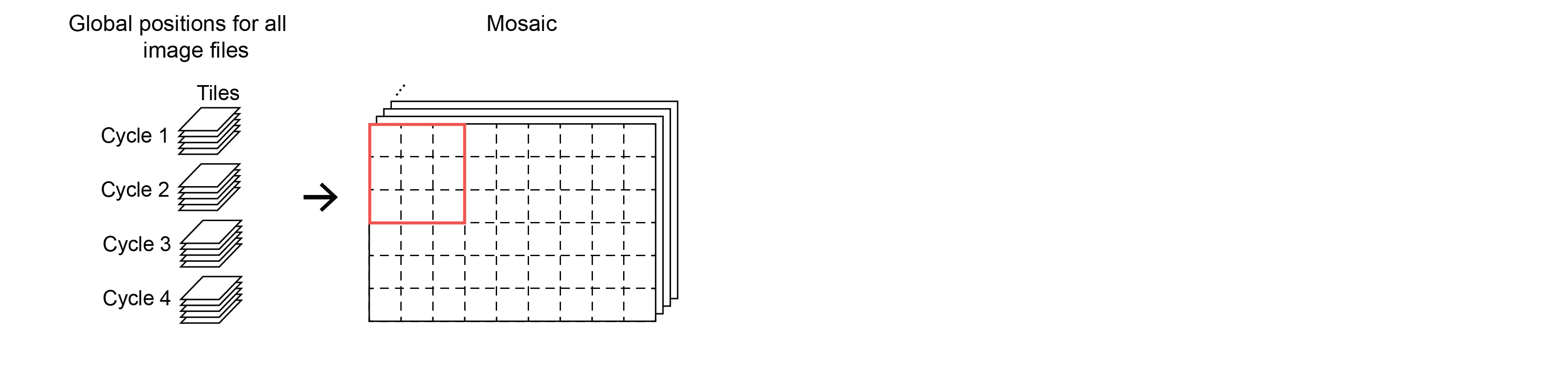
3.1 Create empty image large enough for full data set
To generate the final output image mosaic, we create an empty image large enough to encompass all corrected tile positions and copy each tile into it at the appropriate coordinates.
3.2 Input tile position data
Since each pairwise image registration is computed to a precision of 0.1 pixels as described above, adding up several of these shifts to determine the final coordinates for a given tile generally yields non-integer values. ASHLAR defaults to applying sub-pixel translations on the tile images to account for this, but some users may prefer to round the final positions to the nearest pixel instead.
3.3 Combine overlapping regions with linear blending
Where neighboring image tiles overlap in the mosaic, they are combined with linear blending or one of several other user- selected blending functions.
3.4 Output mosaic image
The final many-channel image is then written out as a standard OME- TIFF file containing a multi-resolution image pyramid to support efficient visualization.