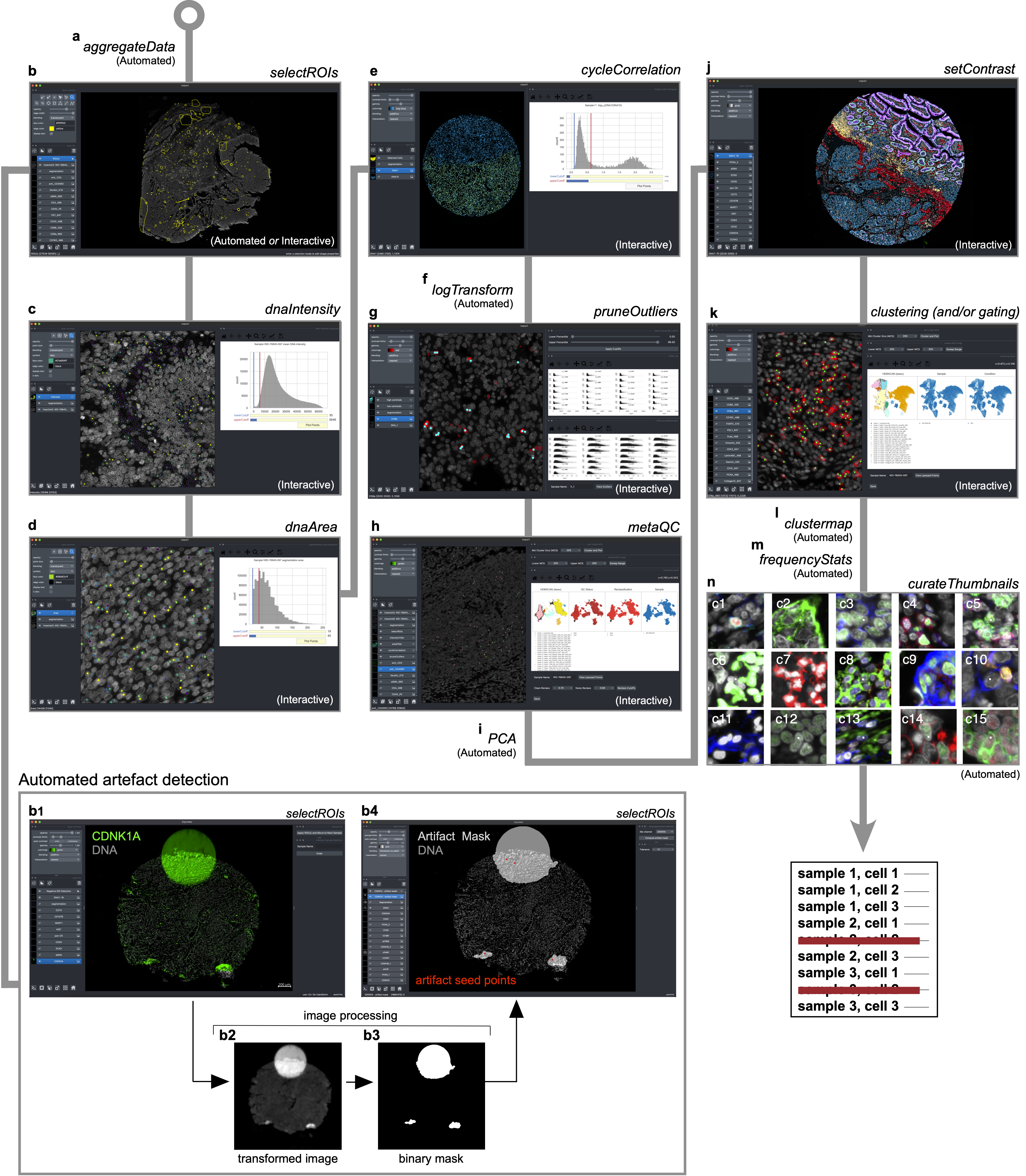
 | Identifying and removing noisy single-cell data points with CyLinter. | CyLinter input consists of multiplex microscopy files (OME-TIFF/TIFF) and their corresponding cell segmentation outlines (OME-TIFF/TIFF), cell ID masks (OME-TIFF/TIFF), and single-cell feature tables (CSV). a, Aggregate data (automated): raw spatial feature tables for all samples in a batch are merged into a single Pandas (Python) dataframe. b, ROI selection (interactive or automated): multi-channel images are viewed to identify and gate on regions of tissue affected by microscopy artefacts (negative selection mode) or areas of tissue devoid of artefacts (positive selection mode. b1-b4, Demonstration of automated artefact detection in CyLinter: b1, CyLinter’s selectROIs module showing artefacts in the CDKN1A (green) channel of a mesothelioma TMA core. b2, Transformed version of the original CDKN1A image such that artefacts appear as large, bright regions relative to channel intensity variations associated with true signal of immunoreactive cells which are suppressed. b3, Local intensity maxima are identified in the transformed image and a flood fill algorithm is used to create a pixel-level binary mask indicating regions of tissue affected by artefacts. In this example, the method identifies three artefacts in the image: one fluorescence aberration at the top of the core, and two tissue folds at the bottom of the core. b4, CyLinter’s selectROIs module showing the binary artefact mask (translucent gray shapes) and their corresponding local maxima (red dots) defining each of the three artefacts. c, DNA intensity filter (interactive): histogram sliders are used to define lower and upper bounds on nuclear counterstain single intensity. Cells between cutoffs are visualized as scatter points at their spatial coordinates in the corresponding tissue for gate confirmation or refinement. d, Segmentation area filter (interactive): histogram sliders are used to define lower and upper bounds on cell segmentation area (pixel counts). Cells between cutoffs are visualized as scatter points at their spatial coordinates in the corresponding tissue for gate confirmation or refinement. e, Cross-cycle correlation filter (interactive): applicable to multi-cycle experiments. Histogram sliders are used to define lower and upper bounds on the log-transformed ratio of DNA signals between the first and last imaging cycles. Cells between cutoffs are visualized as scatter points at their spatial coordinates in their corresponding tissues for gate confirmation or refinement. f, Log transformation (automated): single-cell data are log-transformed. g, Channel outliers filter (interactive): the distribution of cells according to antibody signal intensity is viewed for all sample as a facet grid of scatter plots (or hexbin plots) against cell area (y-axes). Lower and upper percentile cutoffs are applied to remove outliers. Outliers are visualized as scatter points at their spatial coordinates in their corresponding tissues for gate confirmation or refinement. h, MetaQC (interactive): unsupervised clustering methods (UMAP or TSNE followed by HDBSCAN clustering) are used to correct for gating bias in prior data filtration modules by thresholding on the percent of each cluster composed of clean (maintained) or noisy (redacted) cells. i, Principal component analysis (PCA, automated): PCA is performed and Horn’s parallel analysis is used to determine the number of PCs associated with non-random variation in the dataset. j, Image contrast adjustment (interactive): channel contrast settings are optimized for visualization on reference tissues which are applied to all samples in the cohort. k, Unsupervised clustering (interactive): UMAP (or TSNE) and HDBSCAN are used to identify unique cell states in a given cohort of tissues. Manual gating can also be performed to identify cell populations. l, Compute clustered heatmap (automated): clustered heatmap is generated showing channel z-scores for identified clusters (or gated populations). m, Compute frequency statistics (automated): pairwise t statistics on the frequency of each identified cluster or gated cell population between groups of tissues specified in CyLinter’s configuration file (cylinter_config.yml, e.g., treated vs. untreated, response vs. no response, etc.) are computed. n, Evaluate cluster membership (automated): cluster quality is checked by visualizing galleries of example cells drawn at random from each cluster identified in the clustering module (panel k). |