Accessing the data
The package contains the training and test datasets described in the paper. You can access them directly via the data() function after loading the package:
Looking at the first few rows and columns gives the general idea of how the data is structured.
dim( MACCSbinary )## [1] 400 152head( MACCSbinary[,1:6] )## Label Drug pubchem_id MACCS(--8) MACCS(-11) MACCS(-13)
## 1 Sensitive lomerizine dihcl 3949 0 0 0
## 2 Sensitive clotrimazole 2812 0 0 0
## 3 Sensitive loratadine 3957 0 0 0
## 4 Sensitive naftopidil 4418 0 0 0
## 5 Sensitive nefazodone 4449 0 0 0
## 6 Sensitive efavirenz 64139 0 0 0The first column, Label, contains annotations for each drug specifying whether the drug is more ("Sensitive") or less ("Resistant") efficacious in the ABC-16 strain, relative to the parental strain. Test data is located in the last 24 rows of MACCSbinary and contains NAs in the Label column:
tail( MACCSbinary[,1:6] )## Label Drug pubchem_id MACCS(--8) MACCS(-11) MACCS(-13)
## 395 <NA> Rapamycin 5284616 0 0 0
## 396 <NA> Staurosporine 44259 0 0 0
## 397 <NA> Tacrolimus 445643 0 0 0
## 398 <NA> Tamoxifen 2733526 0 0 0
## 399 <NA> Tunicamycin 6433557 0 0 0
## 400 <NA> Valinomycin 441139 0 0 0Drug identity is captured in the second (Drug) and third (pubchem_id) columns. All remaining columns contain molecular features, which in this case consist of binary calls on whether a particular MACCS key is present in a drug’s structure.
SMILES representations of drugs
The package also contains SMILES strings for all 400 drugs considered in the paper. These strings are stored as a separate data frame and can also be retrieved using the data() function.
##               Drug pubchem_id
## 1 lomerizine dihcl       3949
## 2     clotrimazole       2812
## 3       loratadine       3957
## 4       naftopidil       4418
## 5       nefazodone       4449
## 6        efavirenz      64139
##                                                      IsomericSMILES
## 1 COC1=C(C(=C(C=C1)CN2CCN(CC2)C(C3=CC=C(C=C3)F)C4=CC=C(C=C4)F)OC)OC
## 2               C1=CC=C(C=C1)C(C2=CC=CC=C2)(C3=CC=CC=C3Cl)N4C=CN=C4
## 3              CCOC(=O)N1CCC(=C2C3=C(CCC4=C2N=CC=C4)C=C(C=C3)Cl)CC1
## 4                 COC1=CC=CC=C1N2CCN(CC2)CC(COC3=CC=CC4=CC=CC=C43)O
## 5        CCC1=NN(C(=O)N1CCOC2=CC=CC=C2)CCCN3CCN(CC3)C4=CC(=CC=C4)Cl
## 6                  C1CC1C#C[C@]2(C3=C(C=CC(=C3)Cl)NC(=O)O2)C(F)(F)F
##                                                     CanonicalSMILES
## 1 COC1=C(C(=C(C=C1)CN2CCN(CC2)C(C3=CC=C(C=C3)F)C4=CC=C(C=C4)F)OC)OC
## 2               C1=CC=C(C=C1)C(C2=CC=CC=C2)(C3=CC=CC=C3Cl)N4C=CN=C4
## 3              CCOC(=O)N1CCC(=C2C3=C(CCC4=C2N=CC=C4)C=C(C=C3)Cl)CC1
## 4                 COC1=CC=CC=C1N2CCN(CC2)CC(COC3=CC=CC4=CC=CC=C43)O
## 5        CCC1=NN(C(=O)N1CCOC2=CC=CC=C2)CCCN3CCN(CC3)C4=CC(=CC=C4)Cl
## 6                     C1CC1C#CC2(C3=C(C=CC(=C3)Cl)NC(=O)O2)C(F)(F)F
Note that we provide both the Isomeric SMILES strings, which preserve stereochemistry information, as well as Canonical SMILES, where this information is stripped. Both sets of SMILES strings were obtained directly from PubChem, using their PUG REST API.
Visualizing the data
Let’s begin by plotting a heatmap that presents and overview of the entire dataset. We will make extensive use of tidy data manipulation. As the first step, we load the appropriate libraries and define a palette for subsequent plots.
library( tidyverse )
library( plotly )
ABCpal <- c("Resistant" = "tomato", "Sensitive" = "steelblue")
Isolate the training data by selecting the set of rows with non-NA labels. HH will contain the matrix to be plotted as the heatmap, while Annot will store labels that will be displayed as an additional annotation bar at the top of the heatmap. The plotting is done using the pheatmap package.
Xtrain <- MACCSbinary %>% filter( !is.na(Label) )
HH <- Xtrain %>% select(-Label, -Drug) %>% column_to_rownames("pubchem_id") %>% as.matrix
Annots <- select( Xtrain, pubchem_id, Label ) %>% column_to_rownames( "pubchem_id" )
pheatmap::pheatmap( t(HH), show_rownames=FALSE, show_colnames=FALSE,
         annotation_col=Annots, annotation_names_col=FALSE, legend=FALSE,
         color=c("gray90","gray30"), annotation_colors=list(Label=ABCpal) )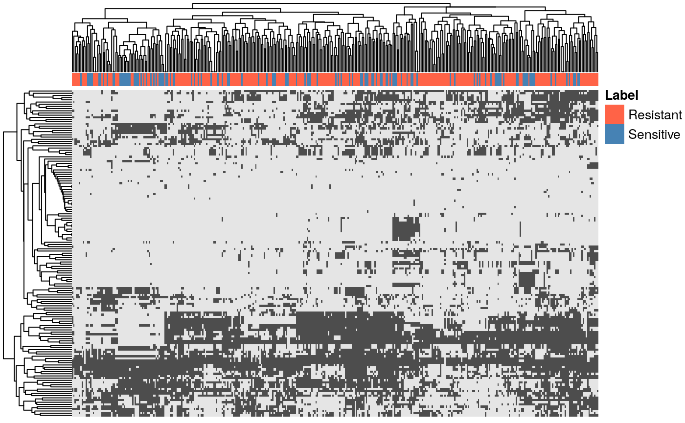
The version of this figure in the paper includes additional post-processing consisting of leaf order optimization and grouping of rows.
Dimensionality reduction
Lastly, we can perform dimensionality reduction to explore the general trends in the data.
## Compute PCA
P <- Xtrain %>% select( -Label, -Drug, -pubchem_id ) %>% prcomp() %>%
    broom::augment( Xtrain ) %>% select( Label, PC1=.fittedPC1, PC2=.fittedPC2 )

## Plot the projection onto the first two principal components
gg <- ggplot( P, aes(x=PC1, y=PC2, color=Label) ) + geom_point() +
    theme_bw() + scale_color_manual( values=ABCpal )
ggplotly(gg)
We observe that the unsupervised analysis is unable to distinguish between the class labels. In the next vignette, we will investigate this data in the context of supverised methods.
Additional Feature Spaces
The package includes three additional feature representations of the same 400 drugs: 1) MACCScount, which captures the number of occurrences of each MACCS fingerprint (as opposed to just their presence/absence, as in MACCSbinary); 2) Morgan, which captures ECFP/Morgan representation; and 3) PChem, which consists of physico-chemical properties. All three matrices are in the same format as MACCSbinary, including having the Label column designate class assignment (Sensitive or Resistant) for training data and NA for test samples.
We can load and examine the data using the same functions as those outlined in the previous sections. Here’s a couple of additional examples:
## Load all three datasets
data( MACCScount, Morgan, PChem )

## Identify the highest number of occurrences of MACCS keys
## List the top keys along with which drugs they occur in
MACCScount %>% gather( Key, nOccur, -Label, -Drug, -pubchem_id ) %>% group_by( Key ) %>%
    filter( nOccur == max(nOccur) ) %>% arrange( desc(nOccur) ) %>% ungroup %>% head
## # A tibble: 6 x 5
## Label Drug pubchem_id Key nOccur
## <chr> <chr> <int> <chr> <int>
## 1 Resistant dactinomycin 457193 MACCS(165) 52
## 2 <NA> Imatinib 5291 MACCS(163) 30
## 3 Resistant vinorelbine bitatrate 5311497 MACCS(105) 29
## 4 Resistant dactinomycin 457193 MACCS(150) 26
## 5 Resistant goserelin acetate 5311128 MACCS(156) 23
## 6 <NA> Valinomycin 441139 MACCS(160) 21## Count the total number of occurrences of Morgan keys
## Display the most commonly-occurring keys
Morgan %>% gather( Key, nOccur, -Label, -Drug, -pubchem_id ) %>% group_by( Key ) %>%
summarize( nTotal = sum(nOccur) ) %>% arrange( desc(nTotal) ) %>% head## # A tibble: 6 x 2
## Key nTotal
## <chr> <int>
## 1 M668 388
## 2 M175 366
## 3 M991 299
## 4 M298 291
## 5 M1241 282
## 6 M1398 280## We may be interested in normalizing each physicochemical property
## to have zero mean and standard deviation of one
PChemNorm <- PChem %>% mutate_at( vars(-Label, -Drug, -pubchem_id), ~(.x - mean(.x))/sd(.x) )
summary( PChemNorm$SlogP )## Min. 1st Qu. Median Mean 3rd Qu. Max.
## -5.68595 -0.57200 0.02156 0.00000 0.62647 3.36914sd( PChemNorm$SlogP )## [1] 1